If Function | And Function | Or Function | Nested If | Ifs | Switch | Roll the Dice
Learn how to use Excel’s logical functions such as the IF, AND and OR function.
If Function
The IF function checks whether a condition is met, and returns one value if TRUE and another value if FALSE.
1. Select cell C2 and enter the following function.
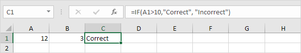
The IF function returns Correct because the value in cell A1 is higher than 10.
And Function
The AND Function returns TRUE if all conditions are true and returns FALSE if any of the conditions are false.
1. Select cell D2 and enter the following formula.
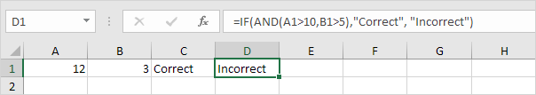
The AND function returns FALSE because the value in cell B2 is not higher than 5. As a result the IF function returns Incorrect.
Or Function
The OR function returns TRUE if any of the conditions are TRUE and returns FALSE if all conditions are false.
1. Select cell E2 and enter the following formula.
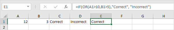
The OR function returns TRUE because the value in cell A1 is higher than 10. As a result the IF function returns Correct.
General note: the AND and OR function can check up to 255 conditions.
Nested If
The IF function in Excel can be nested, when you have multiple conditions to meet. The FALSE value is being replaced by another IF function to make a further test.
Note: if you have Excel 2016, simply use the IFS function.
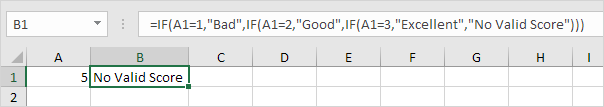
1a. If cell A1 equals 1, the formula returns Bad.
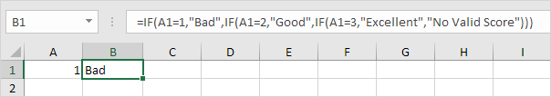
1b. If cell A1 equals 2, the formula returns Good.

1c. If cell A1 equals 3, the formula returns Excellent.
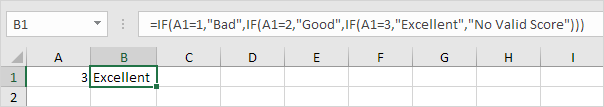
1d. If cell A1 equals another value, the formula returns No Valid Score.
Here’s another example.
2a. If cell A1 is less or equal to 10, the formula returns 350.

2b. If cell A1 is greater than 10 and less or equal to 20, the formula returns 700.


2c. If cell A1 is greater than 20 and less or equal to 30, the formula returns 1400.

2d. If cell A1 is greater than 30, the formula returns 2000.

Note: to slightly change the boundaries, you might want to use “<” instead of “<=” in your own formula.
Ifs Function
Use the IFS function in Excel 2016 when you have multiple conditions to meet. The IFS function returns a value corresponding to the first TRUE condition.
Note: if you don’t have Excel 2016, you can nest the IF function.
1a. If cell A1 equals 1, the IFS function returns Bad.

1b. If cell A1 equals 2, the IFS function returns Good.
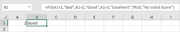
1c. If cell A1 equals 3, the IFS function returns Excellent.

1d. If cell A1 equals another value, the IFS function returns No Valid Score.

Note: instead of TRUE, you can also use 1=1 or something else that is always TRUE.
Here’s another example.
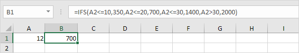
2a. If cell A1 is less or equal to 10, the IFS function returns 350.

2b. If cell A1 is greater than 10 and less or equal to 20, the IFS function returns 700.

2c. If cell A1 is greater than 20 and less or equal to 30, the IFS function returns 1400.
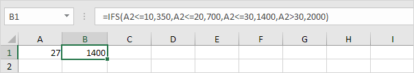
2d. If cell A1 is greater than 30, the IFS function returns 2000.

Note: to slightly change the boundaries, you might want to use “<” instead of “<=” in your own function.
Switch Function
This example teaches you how to use the SWITCH function in Excel 2016 instead of the IFS function.
1a. For example, the IFS function below finds the correct states.
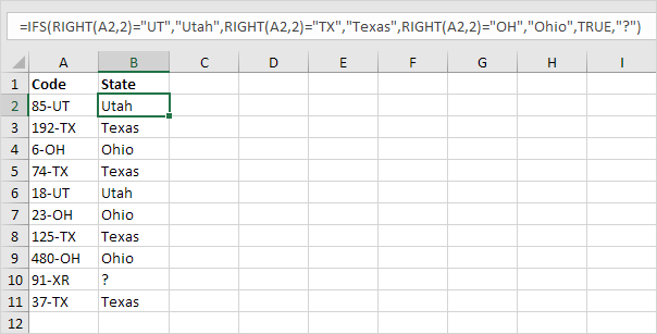
Explanation: cell A2 contains the string 85-UT. The RIGHT function extracts the 2 rightmost characters from this string (UT). As a result, the IFS function returns the correct state (Utah). If the 2 rightmost characters are not equal to UT, TX or OH, the IFS function returns a question mark. Instead of TRUE, you can also use 1=1 or something else that is always TRUE.
1b. The SWITCH function below produces the exact same result but is much easier to read.
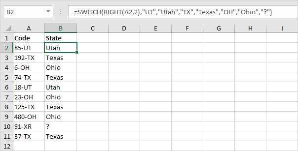
Explanation: if the first argument (RIGHT(A2,2) in this example) equals UT, the SWITCH function returns Utah. If TX, Texas. If OH, Ohio. The last argument (a question mark in this example) is always the default value (if there’s no match).
2. Why not always use the SWITCH function in Excel? There are many examples where you cannot use the SWITCH function instead of the IFS function.

Explanation: because we use”<=” and “>” symbols in this IFS function, we cannot use the SWITCH function.
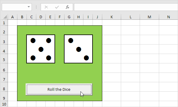
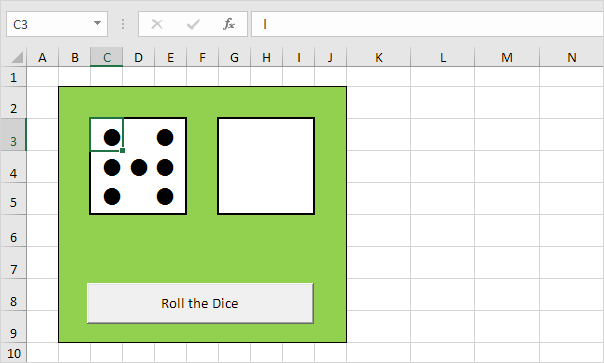
Roll the Dice
This example teaches you how to simulate the roll of two dice in Excel. If you are in a hurry, simply download the Excel file.
Note: the instructions below do not teach you how to format the worksheet. We assume that you know how to change font sizes, font styles, insert rows and columns, add borders, change background colors, etc.
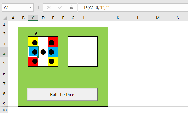
1. At the moment, each cell contains the letter l (as in lion). With a Wingdings font style, these l’s look like dots.
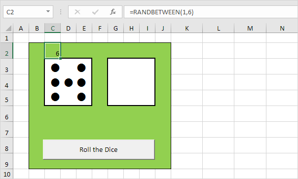
2. Enter the RANDBETWEEN function in cell C2.
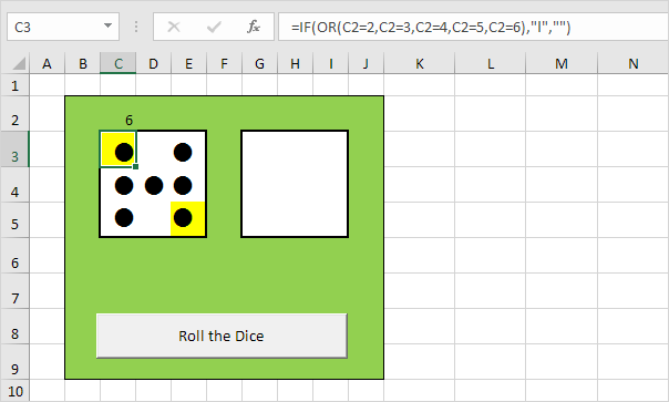
3. Enter the formula shown below into the yellow cells. If we roll 2, 3, 4, 5 or 6, these cells should contain a dot.
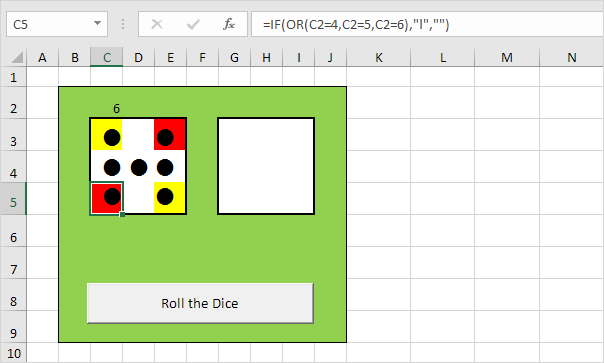
4. Enter the formula shown below into the red cells. If we roll 4, 5 or 6, these cells should contain a dot.
5. Enter the formula shown below into the blue cells. If we roll 6, these cells should contain a dot.
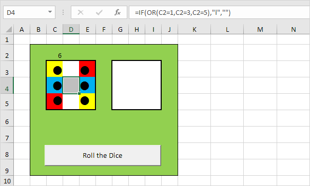
6. Enter the formula shown below into the gray cell. If we roll 1, 3 or 5, this cell should contain a dot.
7. Copy the range C2:E5 and paste it to the range G2:I5.
8. Change the font color of cell C2 and cell G2 to green (so the numbers are not visible).
9. Click the command button on the sheet (or press F9).
Result.