

Year, Month, Day | Date Function | Current Date & Time | Hour, Minute, Second | Time Function | DateDif | weekdays | Time Sheet | Days until Birthday | Last Day of the Month | Holidays | Day of the Year | Quarter
To enter a date in Excel, use the “/” or “-” characters. To enter a time, use the “:” (colon). You can also enter a date and a time in one cell.
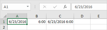

Note: Dates are in US Format. Months first, Days second. This type of format depends on your windows regional settings. Learn more about Date and Time formats.
Year, Month, Day
To get the year of a date, use the YEAR function.
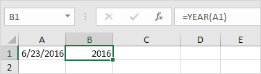
Note: use the MONTH and DAY function to get the month and day of a date.
Date Function
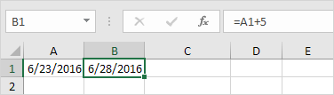
1. To add a number of days to a date, use the following simple formula.
2. To add a number of years, months and/or days, use the DATE function.
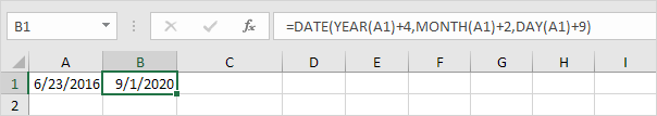

Note: the DATE function accepts three arguments: year, month and day. Excel knows that 6 + 2 = 8 = August has 31 days and rolls over to the next month (23 August + 9 days = 1 September).
Current Date & Time
To get the current date and time, use the NOW function.
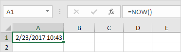

Note: use the TODAY function to get the current date only. Use NOW()-TODAY() to get the current time only (and apply a Time format).
Hour, Minute, Second
To return the hour, use the HOUR function.
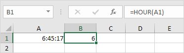
Note: use the MINUTE and SECOND function to return the minute and second.
Time Function
To add a number of hours, minutes and/or seconds, use the TIME function.
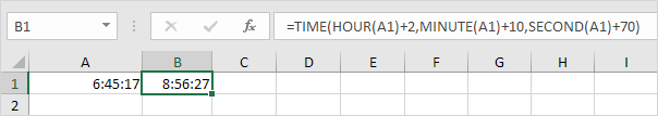
Note: Excel adds 2 hours, 10 + 1 = 11 minutes and 70 – 60 = 10 seconds.
DateDif Function
To get the number of days, weeks or years between two dates in Excel, use the DATEDIF function. The DATEDIF function has three arguments.
1. Fill in “d” for the third argument to get the number of days between two dates.
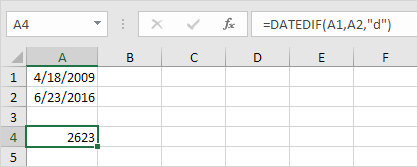

Note: =A2-A1 produces the exact same result!
2. Fill in “m” for the third argument to get the number of months between two dates.

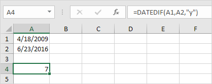
3. Fill in “y” for the third argument to get the number of years between two dates.
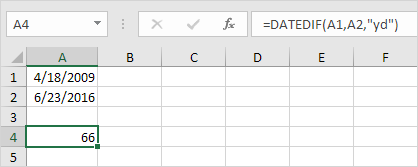
4. Fill in “yd” for the third argument to ignore years and get the number of days between two dates.
5. Fill in “md” for the third argument to ignore months and get the number of days between two dates.

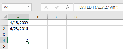
6. Fill in “ym” for the third argument to ignore years and get the number of months between two dates.
Important note: the DATEDIF function returns the number of complete days, months or years. This may give unexpected results when the day/month number of the second date is lower than the day/month number of the first date. See the example below.
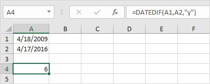
The difference is 6 years. Almost 7 years! Use the following formula to return 7 years.

Weekdays
Weekday Function | Networkdays function | Workday function
Learn how to get the day of the week of a date in Excel and how to get the number of weekdays/working days between two dates.
Weekday Function
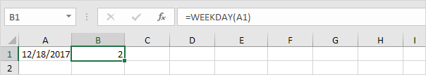
1. The WEEKDAY function in Excel returns a number from 1 (Sunday) to 7 (Saturday) representing the day of the week of a date. Apparently, 12/18/2017 falls on a Monday.
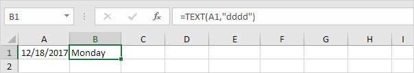
2. You can also use the TEXT function to display the day of the week.
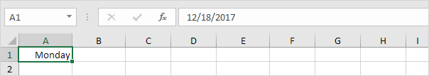
3. Create a custom date format (dddd) to display the day of the week.
Networkdays Function
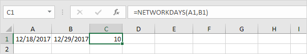
1. The NETWORKDAYS function returns the number of weekdays (weekends excluded) between two dates.
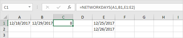
2. If you supply a list of holidays, the NETWORKDAYS function returns the number of workdays (weekends and holidays excluded) between two dates.

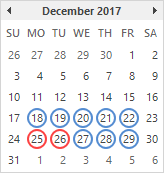
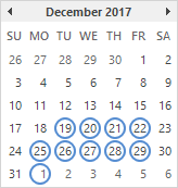
The calendar below helps you understand the NETWORKDAYS function.

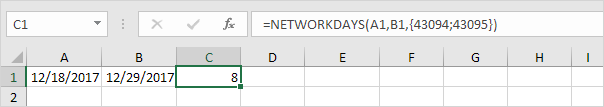
3. Dates are stored as numbers in Excel and count the number of days since January 0, 1900. Instead of supplying a list, supply an array constant of the numbers that represent these dates. To achieve this, select E1:E2 in the formula and press F9.
Workday Function
The WORKDAY function is (almost) the opposite of the NETWORKDAYS function. It returns the date before or after a specified number of weekdays (weekends excluded).
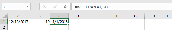
Note: the WORKDAY function returns the serial number of the date. Apply a Date format to display the date.
The calendar below helps you understand the WORKDAY function.
Again, if you supply a list of holidays, the WORKDAY function returns the date before or after a specified number of workdays (weekends and holidays excluded).
Time Sheet
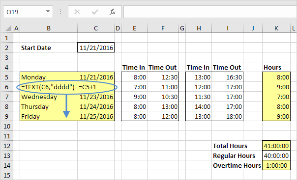
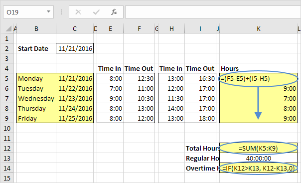
This example teaches you how to create a simple timesheet calculator in Excel. Cells that contain formulas are colored light yellow. If you are in a hurry, simply download the Excel file.
1. To automatically calculate the next 4 days and dates when you enter a start date, use the formulas below.

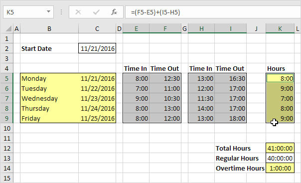
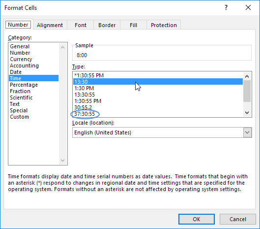
2. Select the cells containing the times.
3. Right click, click Format Cells, and select the right Time format. Use the circled format for cell K12, K13, K14.

4. To automatically calculate the hours worked each day, the total hours and the overtime hours, use the formulas below.
Days until Birthday
To calculate the number of days until your birthday in Excel, execute the following steps.
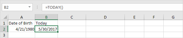
1. Select a cell and enter your date of birth.
2. Select the cell next to it and enter the TODAY function to return today’s date.
3. The most difficult part in order to get the number of days until your birthday is to find your next birthday. The formula below does the trick.
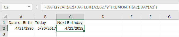
Explanation: The DATE function accepts three arguments: year, month and day. We used the DATEDIF function to find the number of complete years (“y”) between Date of Birth and Today. DATEDIF(A2,B2,”y”) equals 37. If 37 complete years have passed since your date of birth (in other words, you have already celebrated your 37st birthday), your next birthday will be 37 + 1 = 38 years after your date of birth.
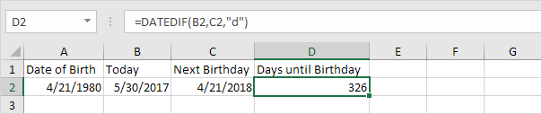
4. Next, we use the DATEDIF function to find the number of days (“d”) between Today and Next Birthday.
Last Day of the Month
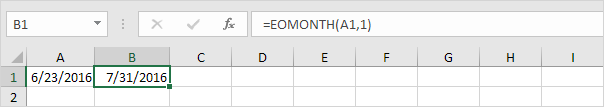
To get the date of the last day of the month in Excel, use the EOMONTH (End of Month) function.
1. For example, get the date of the last day of the current month.

Note: the EOMONTH function returns the serial number of the date. Apply a Date format to display the date.
2. For example, get the date of the last day of the next month.
3. For example, get the date of the last day of the current month – 8 months = 6 – 8 = -2 = October (-2+12=10), 2015!

Holidays
This example teaches you how to get the date of a holiday for any year (2017, 2018, etc). If you are in a hurry, simply download the Excel file.
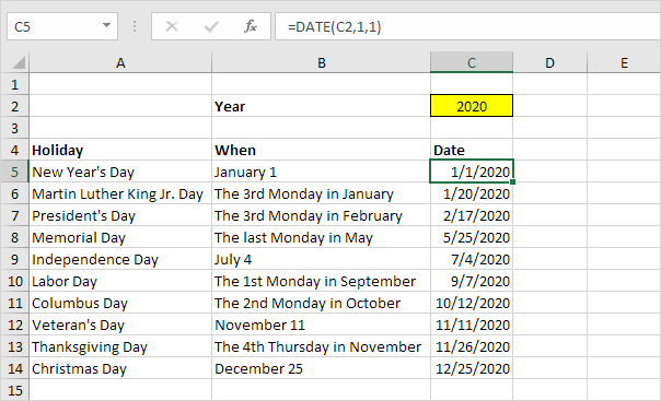
Before you start: the CHOOSE function returns a value from a list of values, based on a position number. For example, =CHOOSE(3,”Car”,”Train”,”Boat”,”Plane”) returns Boat. The WEEKDAY function returns a number from 1 (Sunday) to 7 (Saturday) representing the day of the week of a date.
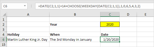
1. This is what the spreadsheet looks like. If you enter a year into cell C2, Excel returns all the holidays for that year. Of course, New Year’s Day, Independence Day, Veteran’s Day and Christmas Day are easy.
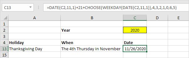
2. All other holidays can be described in a similar way: the xth day in a month (except Memorial day which is slightly different). Let’s take a look at Thanksgiving Day. If you understand Thanksgiving Day, you understand all holidays. Thanksgiving is celebrated the 4th Thursday in November.
The calendar below helps you understand Thanksgiving Day 2020.
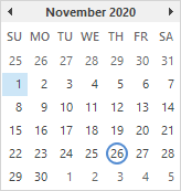
Explanation: DATE(C2,11,1) reduces to 11/1/2020. WEEKDAY(DATE(C2,11,1)) reduces to 1 (Sunday). Now the formula reduces to 11/1/2020 + 21 + CHOOSE(1,4,3,2,1,0,6,5) = 11/1/2020 + 21 + 4 = 11/26/2020. We needed the 4 extra days because it takes 4 days until the first Thursday in November. From there, it takes another 21 days (3 weeks) until the 4rd Thursday in November. It doesn’t matter on which day November 1 falls, the CHOOSE function correctly adds the number of days until the first Thursday in November (notice the pattern in the list of values). From there, it always takes another 21 days until the 4rd Thursday in November. Therefore, this formula works for every year.
3. Let’s take a look at Martin Luther King Jr. Day. This formula is almost the same. Martin Luther King Jr. Day is celebrated the 3rd Monday in January. The first DATE function reduces to the first of January this time. The base position (0) in the list of values for the CHOOSE function is located at the second spot now (we are looking for a Monday)

The calendar below helps you understand Martin Luther King Jr. Day 2020.
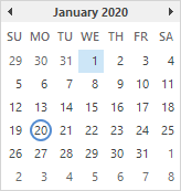
Explanation: DATE(C2,1,1) reduces to 1/1/2020. WEEKDAY(DATE(C2,1,1)) reduces to 4 (Wednesday). Now the formula reduces to 1/1/2020 + 14 + CHOOSE(4,1,0,6,5,4,3,2) = 1/1/2020 + 14 + 5 = 1/20/2020. We needed the 5 extra days because it takes 5 days until the first Monday in January.
Day of the Year
An easy formula that returns the day of the year for a given date. There’s no built-in function in Excel that can do this.
1. Enter the formula shown below.
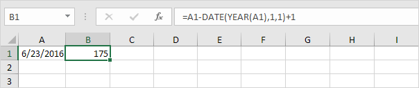
Explanation: Dates and times are stored as numbers in Excel and count the number of days since January 0, 1900. June 23, 2016 is the same as 42544. The DATE function accepts three arguments: year, month and day. DATE(YEAR(A1),1,1) or 1-jan-2016 is the same as 42370. Subtracting these numbers (42544 – 42370 = 174) and adding 1 gives the day of the year.
Quarter
An easy formula that returns the quarter for a given date. There’s no built-in function in Excel that can do this.
1. Enter the formula shown below.
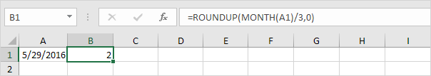
Explanation: ROUNDUP(x,0) always rounds x up to the nearest integer. The MONTH function returns the month number of a date. In this example, the formula reduces to =ROUNDUP(5/3,0), =ROUNDUP(1.666667,0), 2. May is in Quarter 2.
2. Let’s see if this formula works for all months.
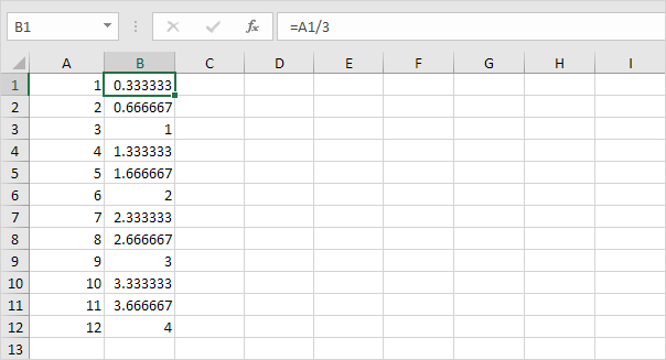

Explanation: now it’s not difficult to see that the first three values (months) in column B are rounded up to 1 (Quarter 1), the next three values (months) in column B are rounded up to 2 (Quarter 2), etc.