SPSS binomial test is used for testing whether a proportion from a single dichotomous variable is equal to a presumed population value. The figure illustrates the basic idea.
SPSS Binomial Test Example
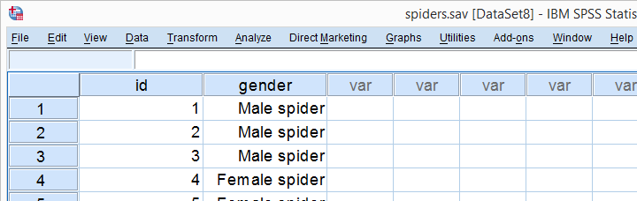
A biologist claims that 75% of a population of spiders consist of female spiders. With a lot of effort he collects 15 spiders, 7 of which are female. These data are in spiders.sav, part of which are shown below.
1. Quick Data Check
Let’s first take a quick look at the FREQUENCIES for gender. Like so, we can inspect whether there are any missing values and whether the variable is really dichotomous. We’ll run some FREQUENCIES. The syntax is so simple that we’ll just type it instead of clicking through the menu.
frequencies gender.

The output tells us that there are no missing values and the variable is indeed dichotomous. We can proceed our analysis with confidence.
2. Assumptions Binomial Test
The results from any statistical test can only be taken seriously insofar as its assumptions have been met. For the binomial test we need just one:
- independent observations (or, more precisely, independent and identically distributed variables);
This assumption is beyond the scope of this tutorial. We presume it’s been met by the data at hand.
3. Run SPSS Binomial Test
We’d like to test whether the proportion of female spiders differs from .75 (our test proportion). Now SPSS Binomial Test has a very odd feature: the test proportion we enter applies to the category that’s first encountered in the data. So the hypothesis that’s tested depends on the order of the cases. Because our test proportion applies to female (rather than male) spiders, we need to move our female spiders to the top of the data file. We’ll do so by running the syntax below. Next, we’ll run the actual binomial test.
sort cases by gender.

 Clicking results in the syntax below. We’ll run it and move on the the output.
NPAR TESTS
/BINOMIAL (.75)=gender
/MISSING ANALYSIS.
4. SPSS Binomial Test Output

 Since we have 7 female spiders out of 15 observations, the observed proportion is (7 / 15 =) .47.
 Our null hypothesis states that this proportion is .75 for the entire population.
 The p value, denoted by Exact Sig. (1-tailed) is .017. If the proportion of female spiders is exactly .75 in the entire population, then there’s only a 1.7% chance of finding 7 or fewer female spiders in a sample of N = 15. We often reject the null hypothesis if this chance is smaller than 5% (p < .05). We conclude that the proportion of female spiders is not .75 in the population but probably (much) lower.
Note that the p value is the chance of finding the observed proportion or a “more extreme” outcome. If the observed proportion is smaller than the test proportion, then a more extreme outcome is an even smaller proportion than the one we observe. We ignore the fact that finding very large proportions would also contradict our null hypothesis. This is what’s meant by (1-tailed).
5. Reporting a Binomial Test
When reporting test results, we always report some descriptive statistics as well. In this case, a frequency table will do. Regarding the significance test, we’ll write something like “a binomial test indicated that the proportion of female spiders of .47 was lower than the expected .75, p = .017 (1-sided)”.