SPSS Sign Test for One Median – Simple Example

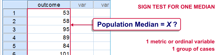
A sign test for one median is often used instead of a one sample t-test when the latter’s assumptions aren’t met by the data. The most common scenario is analyzing a variable which doesn’t seem normally distributed with few (say n < 30) observations. *

This tutorial shows how to run and interpret a sign test in SPSS. We’ll use adratings.sav throughout, part of which is shown below.

SPSS Sign Test – Null Hypothesis

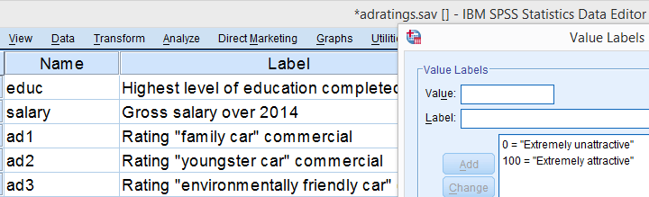
A car manufacturer had 3 commercials rated on attractiveness by 18 people. They used a percent scale running from 0 (extremely unattractive) through 100 (extremely attractive). A marketeer thinks a commercial is good if at least 50% of some target population rate it 80 or higher.

Now, the score that divides the 50% lowest from the 50% highest scores is known as the median. In other words, 50% of the population scoring 80 or higher is equivalent to our null hypothesis thatthat the population median is at least 79.5 for each commercial.If this is true, then the medians in our sample will be somewhat different due to random sampling fluctuation. However, if we find very different medians in our sample, then our hypothesized 79.5 population median is not credible and we’ll reject our null hypothesis.

Quick Data Check – Histograms

Let’s first take a quick look at what our data look like in the first place. We’ll do so by inspecting histograms over our outcome variables by running the syntax below.

Result

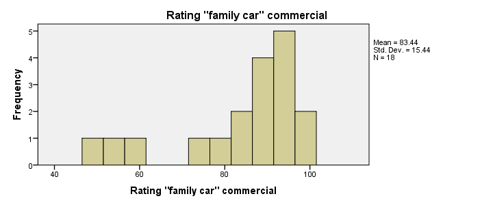
First, note that all distributions look plausible. Since n = 18 for each variable, we don’t have any missing values. The distributions don’t look much like normal distributions. Combined with our small sample sizes, this violates the normality assumption required by t tests so we probably shouldn’t run those.

Quick Data Check – Medians

Our histograms included mean scores for our 3 outcome variables but what about their medians? Very oddly, we can’t compute medians -which are descriptive statistics- with DESCRIPTIVES. We could use FREQUENCIES but we prefer the table format we get from MEANS as shown below.

SPSS – Compute Medians Syntax

Result

Only our first commercial (“family car”) has a median close to 79.5. The other 2 commercials have much lower median. But are they different enough for rejecting our null hypothesis? We’ll find out in a minute.

SPSS Sign Test – Recoding Data Values

SPSS includes a sign test for two related medians but the sign test for one median is absent. But remember that our null hypothesis of a 79.5 population median is equivalent to 50% of the population scoring 80 or higher. And SPSS does include a test for a single proportion (a percentage divided by 100) known as the binomial test. We’ll therefore just use binomial tests for evaluating if the proportion of respondents rating each commercial 80 or higher is equal to 0.50.

The easy way to go here is to RECODE our data values: values smaller than the hypothesized population median are recoded into a minus (-) sign.

Values larger than this median get a plus (+) sign. It’s these plus and minus signs that give the sign test its name. Values equal to the median are excluded from analysis so we’ll specify them as missing values.

SPSS RECODE Syntax

SPSS Binomial Test Menu

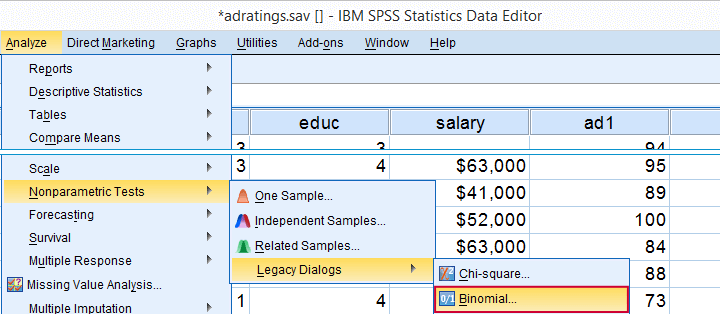
Minor note: the binomial test is a test for a single proportion, which is a population parameter. So it’s clearly not a nonparametric test.

Unfortunately, “nonparametric tests” often refers to both nonparametric and distribution free tests -even though these are completely different things.

 t1 is one of our newly created variables. It merely indicates if ad1 was 80 or higher. Completing the steps results in the syntax below.

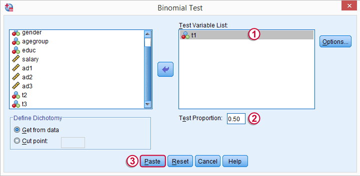
SPSS Binomial Test Syntax

Modifying Our Syntax

Oddly, SPSS’ binomial test results depend on the (arbitrary) order of cases: the test proportion applies to the first value encountered in the data. This is no major issue if -and only if- our test proportion is 0.50 but it still results in messy output. We’ll avoid this by sorting our cases on each test variable before each test.

Modified Binomial Test Syntax

Binomial Test Output

We’ll first limit our focus to the first table of test results as shown below.

 N: 5 out of 18 cases score higher than 79.5;
 the observed proportion is (5 / 18 =) 0.28 or 28%;
 the hypothesized test proportion is 0.50;
 p (denoted as “Exact Significance (2-tailed)”) = 0.096: the probability of finding our sample result is roughly 10% if the population proportion really is 50%. We generally reject our null hypothesis if p < 0.05 soour binomial test does not refute the hypothesis that our population median is 79.5.Before we move on, let’s take a close look at what our 2-tailed significance level of 0.096 really means.

The Binomial Distribution

Statistically, drawing 18 respondents from a population in which 50% scores 80 or higher is similar to flipping a balanced coin 18 times in a row: we could flip anything between 0 and 18 heads. If we repeat our 18 coin flips over and over again, the sampling distribution of the number of heads will closely resemble the binomial distribution shown below.

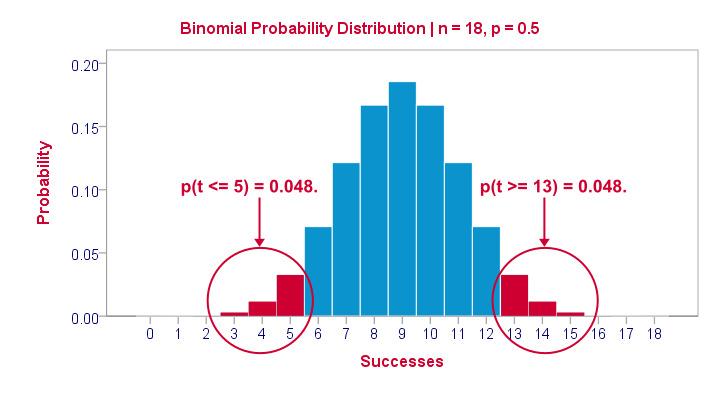
The most likely outcome is 9 heads with a probability around 0.19 or 19%. P = 0.048 for outcomes of 5 or fewer heads (red area). Now, reporting this 1-tailed p-value suggests that none of the other outcomes would refute the null hypothesis. This does not hold because 13 or more heads are also highly unlikely. So we should take into account our deviation of 4 heads from the expected 9 heads in both directions and add up their probabilities. This results in our 2-tailed p-value of 0.096.

Binomial Test – More Output

We saw previously that our second commercial (“youngster car”) has a sample median of 55.5. Our p-value of 0.000 means that we’ve a 0% probability of finding this sample median in a sample of n = 18 when the population median is 79.5. Since p < 0.05, we reject the null hypothesis: the population median is not 79.5 but -presumably- much lower. We’ll leave it as an exercise to the reader to interpret the third and final test.

That’s it for now. I hope this tutorial made clear how to run a sign test for one median in SPSS