VLookup | HLookup | Match | Index | Choose
Learn all about Excel’s lookup & reference functions such as the VLOOKUP, HLOOKUP, MATCH, INDEX and CHOOSE function.
VLookup
The VLOOKUP (Vertical lookup) function looks for a value in the leftmost column of a table, and then returns a value in the same row from another column you specify.
1. Insert the VLOOKUP function shown below.
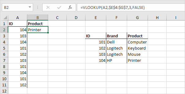
Explanation: the VLOOKUP function looks for the ID (104) in the leftmost column of the range $E$4:$G$7 and returns the value in the same row from the third column (third argument is set to 3). The fourth argument is set to FALSE to return an exact match or a #N/A error if not found.
2. Drag the VLOOKUP function in cell B2 down to cell B11.
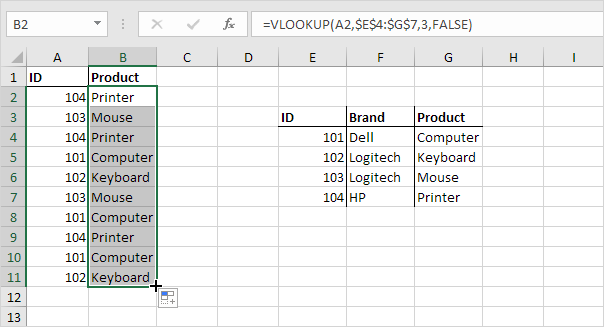
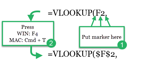
Note: when we drag the VLOOKUP function down, the absolute reference ($E$4:$G$7) stays the same, while the relative reference (A2) changes to A3, A4, A5, etc.
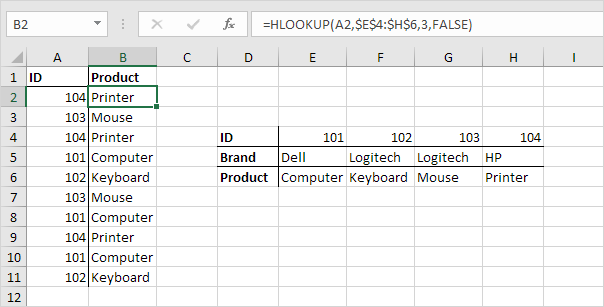
HLookup
In a similar way, you can use the HLOOKUP (Horizontal lookup) function.
Match
The MATCH function returns the position of a value in a given range.
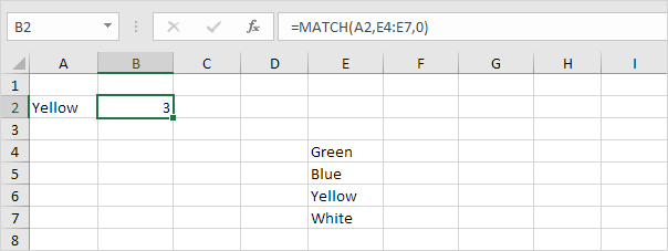
Explanation: Yellow found at position 3 in the range E4:E7. The third argument is optional. Set this argument to 0 to return the position of the value that is exactly equal to lookup_value (A2) or a #N/A error if not found.
Index
The INDEX function below returns a specific value in a two-dimensional range.
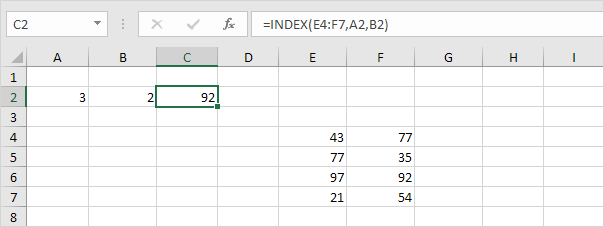
Explanation: 92 found at the intersection of row 3 and column 2 in the range E4:F7.
The INDEX function below returns a specific value in a one-dimensional range.
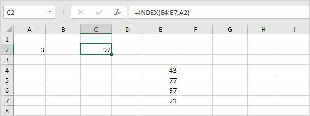
Explanation: 97 found at position 3 in the range E4:E7.
Choose
The CHOOSE function returns a value from a list of values, based on a position number.
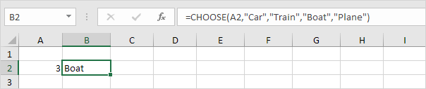
Explanation: Boat found at position 3..
Must See:
Tax Rates
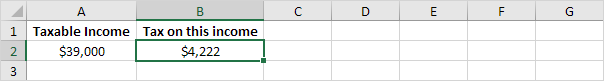
Sometimes you are not looking for an exact match when you use the VLOOKUP function in Excel. For example, when you want to calculate the tax on an income.
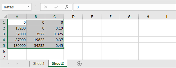
The following tax rates apply to individuals who are residents of Australia.

Example: if income is 39000, tax equals 3572 + 0.325 * (39000 – 37000) = 3572 + 650 = $4222
To automatically calculate the tax on an income, execute the following steps.
1. On the second sheet, create the following range and name it Rates.
2. We already know how the VLOOKUP function can return an exact match or a #N/A error if not found, by setting the fourth argument to FALSE. However, when you set this argument to TRUE, it returns an exact match or if not found, it returns the largest value smaller than lookup_value (A2). That’s exactly what we want!
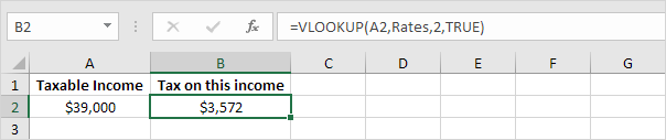
Explanation: Excel cannot find 39000 in the first column of Rates. However, it can find 37000 (the largest value smaller than 39000). As a result, it returns 3572 (col_index_num, the third argument, is set to 2).
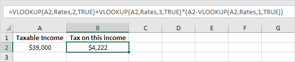
3. Now, what’s left is the remainder of the equation, + 0.325 * (39000 – 37000). This is easy. We can return 0.325 by setting col_index_num to 3 and return 37000 by setting col_index_num to 1. The complete formula below does the trick.
Note: when you set the fourth argument of the VLOOKUP function to TRUE, the first column of the table must be sorted in ascending order.
Offset
The OFFSET function in Excel returns a cell or range of cells that is a specified number of rows and columns from a cell or range of cells.
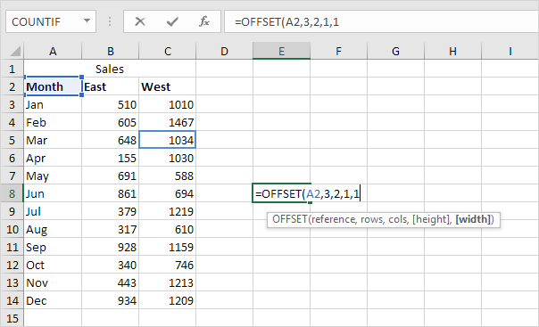
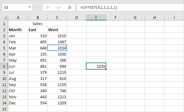
1. The OFFSET function below returns the cell that is 3 rows below and 2 columns to the right of cell A2. The OFFSET function returns a cell because the height and width are both set to 1.
Result:
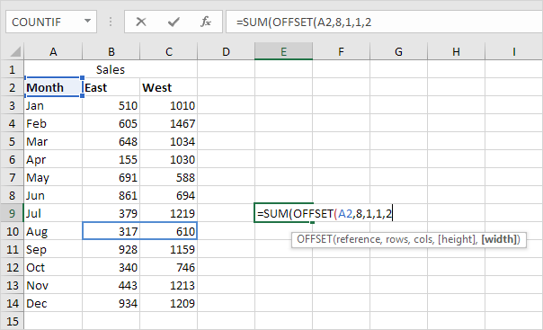
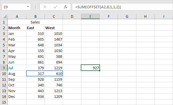
2. The OFFSET function below returns the 1 x 2 range that is 8 rows below and 1 column to the right of cell A2. The SUM function calculates the sum of this range.
Result:
Note: to return a range (without calculating the sum), select a range of the same size before you insert the OFFSET function. If you want to return a cell or range of cells that is a specified number of rows above or columns to the left, enter a negative number.