Relative Reference | Absolute Reference | Mixed Reference | Copy Exact Formula | 3D-reference | External References | Hyperlinks |
Cell references in Excel are very important. Understand the difference between relative, absolute and mixed reference, and you are on your way to success.
Relative Reference
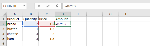
By default, Excel uses relative reference. See the formula in cell D2 below. Cell D2 references (points to) cell B2 and cell C2. Both references are relative.
1. Select cell D2, click on the lower right corner of cell D2 and drag it down to cell D5.
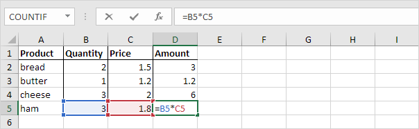
Cell D3 references cell B3 and cell C3. Cell D4 references cell B4 and cell C4. Cell D5 references cell B5 and cell C5. In other words: each cell references its two neighbors on the left.
Absolute Reference
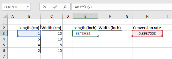
See the formula in cell E3 below.
1. To create an absolute reference to cell H3, place a $ symbol in front of the column letter and row number of cell H3 ($H$3) in the formula of cell E3.
2. Now we can quickly drag this formula to the other cells.
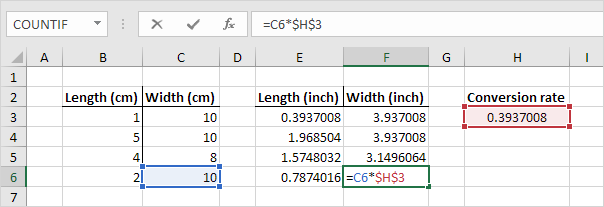
The reference to cell H3 is fixed (when we drag the formula down and across). As a result, the correct lengths and widths in inches are calculated.
Mixed Reference
Sometimes we need a combination of relative and absolute reference (mixed reference).
1. See the formula in cell F2 below.
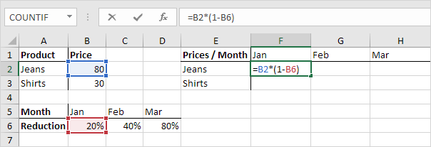
2. We want to copy this formula to the other cells quickly. Drag cell F2 across one cell, and look at the formula in cell G2.
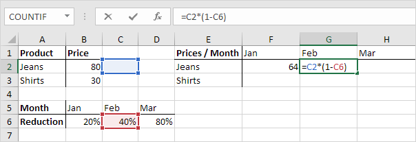
Do you see what happens? The reference to the price should be a fixed reference to column B. Solution: place a $ symbol in front of the column letter of cell B2 ($B2) in the formula of cell F2. In a similar way, when we drag cell F2 down, the reference to the reduction should be a fixed reference to row 6. Solution: place a $ symbol in front of the row number of cell B6 (B$6) in the formula of cell F2.
Result:

Note: we don’t place a $ symbol in front of the row number of B2 (this way we allow the reference to change from B2 (Jeans) to B3 (Shirts) when we drag the formula down). In a similar way, we don’t place a $ symbol in front of the column letter of B6 (this way we allow the reference to change from B6 (Jan) to C6 (Feb) and D6 (Mar) when we drag the formula across).
3. Now we can quickly drag this formula to the other cells.
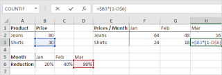
The references to column B and row 6 are fixed.
Copy Exact Formula
When you copy a formula, Excel automatically adjusts the cell references for each new cell the formula is copied to.
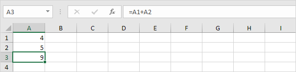
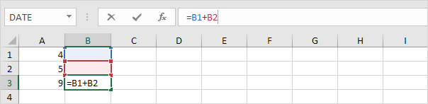
For example, cell A3 below contains a formula which adds the value of cell A2 to the value of cell A1.
When you copy this formula to cell B3 (select cell A3, press CTRL + c, select cell B3, press CTRL + v), the formula will automatically reference the values in column B.
If you don’t want this but instead want to copy the exact formula (without changing the cell references), execute the following easy steps.
1. Click in the formula bar and select the formula.
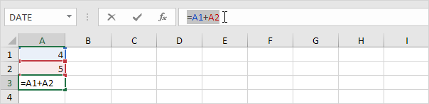
2. Press CTRL + c, and press Enter.
3. Select cell B3 and click in the formula bar again.
4. Press CTRL + v, and press Enter.
Result:
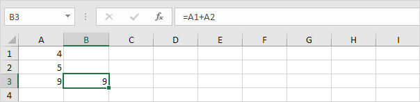
Both cell A3 and cell B3 contain the exact same formula now.
3D-reference
A 3D-reference in Excel refers to the same cell or range on multiple worksheets. First, we’ll look at the alternative.
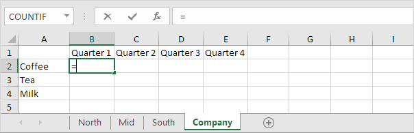
1. On the Company sheet, select cell B2 and type an equal sign =
2. Go to the North sheet, select cell B2 and type a +
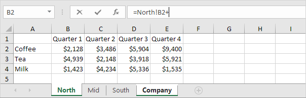
3. Repeat step 2 for the Mid and South sheet.
Result.

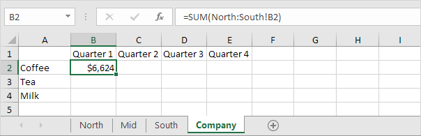
4. This is quite a lot of work. Instead of doing this, use the following 3D-reference: North:South!B2 as the argument for the SUM function.
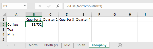
5. If you add worksheets between North and South, this worksheet is automatically included in the formula in cell B2.
External References
Create External Reference | Alert | Edit Links
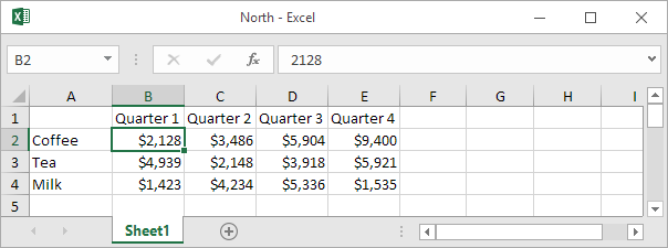
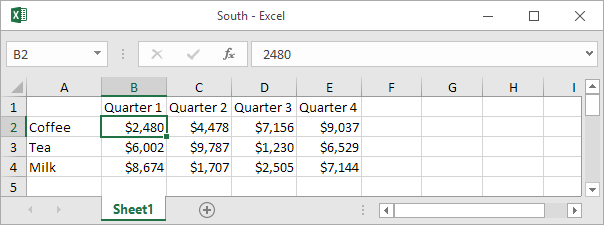
An external reference in Excel is a reference to a cell or range of cells in another workbook. Below you can find the workbooks of three divisions (North, Mid and South).

Create External Reference
To create an external reference, execute the following steps.
1. Open all workbooks.
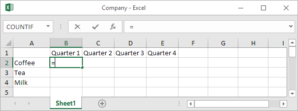
2. In the Company workbook, select cell B2 and type the equal sign =
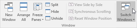
3. On the View tab, in the Window group, click Switch Windows.
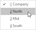
4. Click North.
5. In the North workbook, select cell B2.
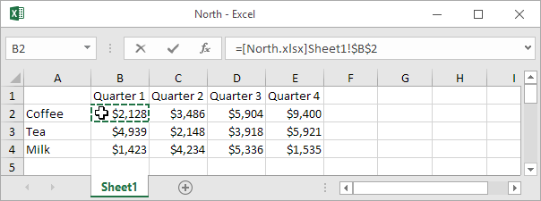
6. Type a +
7. Repeat steps 3 to 6 for the Mid workbook.
8. Repeat steps 3 to 5 for the South workbook.
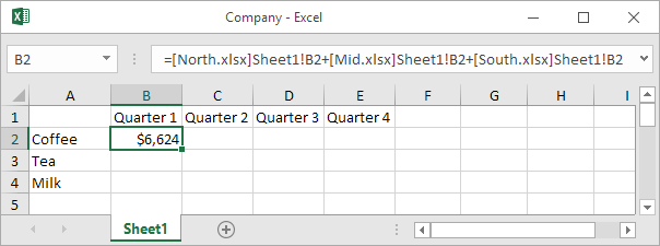
9. Remove the $ symbols in the formula of cell B2.
Result:
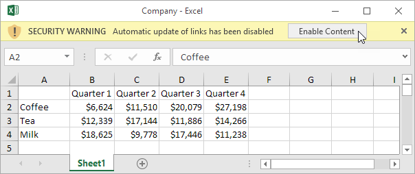
10. Copy the formula to the other cells.
Alert
Close all workbooks. Change a number in the workbook of a division. Close all workbooks again. Open the Company workbook.
A. To update all links, click Enable Content.
B. To not update the links, click the X.
Note: if you see another alert, click Update or Don’t Update.
Edit Links
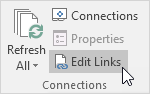
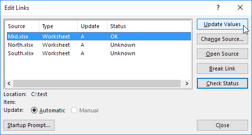
On the Data tab, in the Connections group, click Edit Links to launch the Edit Links dialog box.
1. If you didn’t update the links, you can still update the links here. Select a workbook and click Update Values to update the links to this workbook. Note how the Status changes to OK.
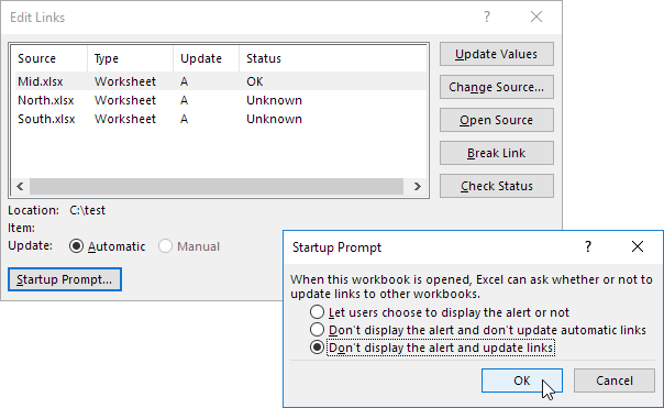
2. If you don’t want to display the alert and update the links automatically, Click Startup Prompt, select the third option, and click OK.
Hyperlinks
Existing File or Web Page | Place in This Document
To create a hyperlink in Excel, execute the following steps.
1. On the Insert tab, in the Links group, click Hyperlink.
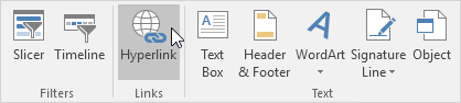
The ‘Insert Hyperlink’ dialog box appears.
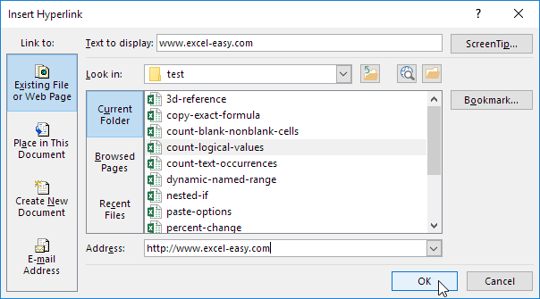
Existing File or Web Page
To create a link to an existing file or web page, execute the following steps.
1a. To create a link to an existing Excel file, select a file (use the Look in drop-down list, if necessary).
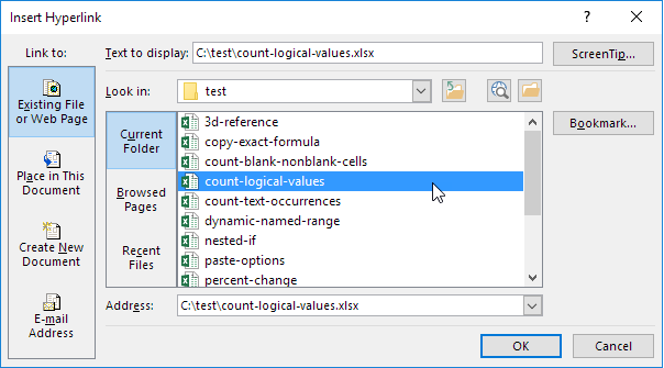
1b. To create a link to a web page, type the Text to display, the Address, and click OK.
Result:
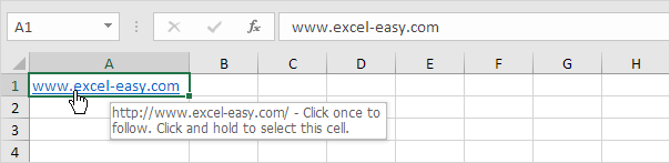
Note: if you want to change the text that appears when you hover over the link, click ScreenTip.
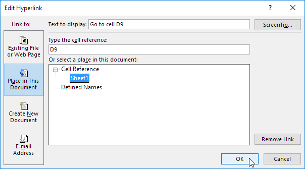
Place in This Document
To create a link to a place in this document, execute the following steps.
1. Click ‘Place in This Document’ under Link to.
2. Type the Text to display, the cell reference, and click OK.
Result:
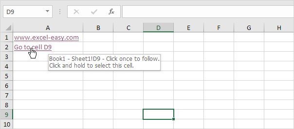
Note: if you want to change the text that appears when you hover over the link, click ScreenTip.