Microsoft Excel introduces powerful XLOOKUP function

Microsoft has introduced a new function in MS Excel – X LOOKUP; A very new and unique function which will replace V LOOKUP. Take a look at Practical Training on X LOOKUP

Use the XLOOKUP function when you need to find things in a table or a range by row. For example, look up the price of an automotive part by the part number, or find an employee name based on their employee ID. With XLOOKUP, you can look in one column for a search term, and return a result from the same row in another column, regardless of which side the return column is on.

Examples

This example is from the video above, and uses a simple XLOOKUP to look up a country name, then return its telephone country code. It only includes the lookup_value (cell F2), lookup_array (range B2:B11), and return_array (range D2:D11) arguments. It does not include the match_mode argument, as XLOOKUP defaults to an exact match.

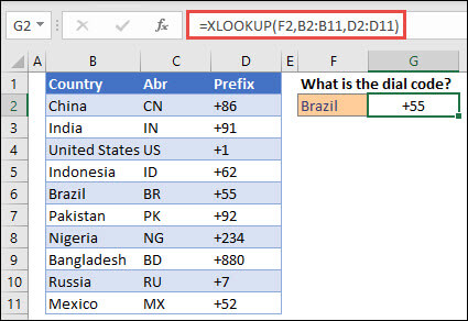
Note: XLOOKUP is different from VLOOKUP in that it uses separate lookup and return arrays, where VLOOKUP uses a single table array followed by a column index number. The equivalent VLOOKUP formula in this case would be: =VLOOKUP(F2,B2:D11,3,FALSE)

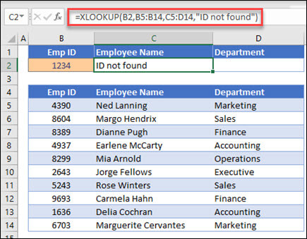
This example adds the if_not_found argument to the example above.

Example of the XLOOKUP function used to return an Employee Name and Department based on Employee ID with the if_not_found argument. The formula is =XLOOKUP(B2,B5:B14,C5:D14,0,1,"Employee not found")

The following example looks in column C for the personal income entered in cell E2, and finds a matching tax rate in column B. It sets the if-not_found argument to return a 0 if nothing is found. The match_mode argument is set to 1, which means the function will look for an exact match, and if it can’t find one, it will return the next larger item. Finally, the search_mode argument is set to 1, which means the function will search from the first item to the last.

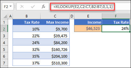
Image of the XLOOKUP function used to return a tax rate based on maximum income. This is an approximate match.The formula is: =XLOOKUP(E2,C2:C7,B2:B7,1,1)

Note: Unlike VLOOKUP, the lookup_array column is to the right of the return_array column, where VLOOKUP can only look from left-to-right.

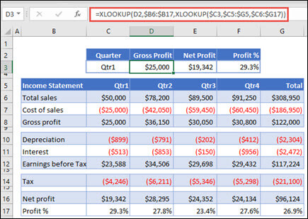Next, we’ll use a nested XLOOKUP function to perform both a vertical and horizontal match. In this case, it will first look for Gross Profit in column B, then look for Qtr1 in the top row of the table (range C5:F5), and return the value at the intersection of the two. This is similar to using the INDEX and MATCH functions in conjunction. You can also use XLOOKUP to replace the HLOOKUP function. Image of the XLOOKUP function used to return horizontal data from a table by nesting 2 XLOOKUPs. The formula is: =XLOOKUP(D2,$B6:$B17,XLOOKUP($C3,$C5:$G5,$C6:$G17))

Image of the XLOOKUP function used to return horizontal data from a table by nesting 2 XLOOKUPs. The formula is: =XLOOKUP(D2,$B6:$B17,XLOOKUP($C3,$C5:$G5,$C6:$G17))

The formula in cells D3:F3 is: =XLOOKUP(D2,$B6:$B17,XLOOKUP($C3,$C5:$G5,$C6:$G17)).

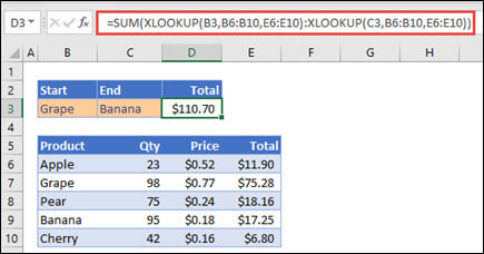
This example uses the SUM function, and two XLOOKUP functions nested together to sum all the values between two ranges. In this case, we want to sum the values for grapes, bananas, and include pears, which are between the two. Using XLOOKUP with SUM to total a range of values that fall between two selections

Using XLOOKUP with SUM to total a range of values that fall between two selections

The formula in cell E3 is: =SUM(XLOOKUP(B3,B6:B10,E6:E10):XLOOKUP(C3,B6:B10,E6:E10))

How does it work? XLOOKUP returns a range, so when it calculates, the formula ends up looking like this: =SUM($E$7:$E$9). You can see how this works on your own by selecting a cell with an XLOOKUP formula similar to this one, then go to Formulas > Formula Auditing > Evaluate Formula, and press the Evaluate button to step through the calculation.

Source: MS Office | Beta News