
XLOOKUP()
Horizontal & Vertical lookup functions
by dw faisalabad
- Introduction
- xlookup and vlookup Limitations
- xlookup and vlookup comparison table
- xlookup Syntax
- Major Differences
- 13 XLOOKUP Examples
- More Emaples
- xlookup vs vlookup vs index/match
- Pros & Cons of XLOOKUP
- Summary
- Conclussion
Introduction
XLOOKUP has defeated Vlookup by introducing eight new features that has increased the working style with MS EXCEL. In this article we are going to take a complete review of Vlookup and Xlookup differences. The XLOOKUP and VLOOKUP functions in Excel are used to find, or ‘lookup’, a value from a table or a list and then return a related result. In this resource, we’ll discuss XLOOKUP vs VLOOKUP with examples of how to use each.
XLOOKUP resolves all of this by replacing the table array parameter with 2 new array parameters – the lookup array and the return array. This simple and elegant change makes everything so much less brittle and so much more dynamic.
Please note that the XLOOKUP function is currently only accessible for Microsoft 365 subscribers.
XLOOKUP V’s VLOOKUP – 8 Limitations Removed
The Following eight new features has been added in XLOOKUP that vlookup has not.[7]
- You cannot carry out an exact lookup by default with VLOOKUP – Guess what? you can with XLOOKUP. Exact lookup is the default setting in the new function.
- You can not look up to the left with VLOOKUP – You can lookup to the left with XLOOKUP. As long as the arrays are of the same size (lookup array and return array), you can really lookup where you want.
- You can’t use VLOOKUP for a horizontal Lookup – You can carry out a horizontal Lookup with XLOOKUP.
- Adding new columns to a table used in a VLOOKUP can break your formula. – You can add as many new columns with XLOOKUP as you like. There is no table array or column index to define in the next XLOOKUP.
- It is not possible to search from bottom to top of a column with VLOOKUP – With XLOOKUP you can search from bottom to top.
- Binary searches using VLOOKUP are not possible – You can with XLOOKUP.
- You cannot carry out an approximate match if the table unless the table is sorted smallest to largest. You can carry out a XLOOKUP without sorting the table. This is an amazing step forward.
- It is not possible to return an approximate match value that is higher using VLOOKUP. You can select to return an approximate match of a value higher with XLOOKUP. You can also select an approximate match of a lower value by default.
XLOOKUP vs VLOOKUP: Comparison table
Xlookup Syntax
Both formulae require a minimum of three arguments. The square brackets indicate the optional arguments [9].
=vlookup(lookup_value, table_array, col_index_num, [range_lookup])
=xlookup(lookup_value, lookup_array, return_array, [if_not_found], [match_mode], [search_mode])
-
lookup_value: this is the value you are searching for
-
lookup_array: this is the range where you are searching for it
-
return_array: this is the range with the result you want
-
[if_not_found]: instead of #N/A, you can specify what should be returned in case no match is found.
-
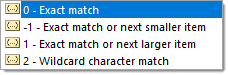
[match_mode]: like with VLOOKUP or INDEX/MATCH, use 0 for an exact match (#N/A will be returned if no match is found). But but but… exact match is the default value, so basically most of the time you won’t need to use this argument! You can also use -1 to return the next smaller value if no match is found, or 1 to return the next larger value if no match is found. It is also possible to use 2, which is a wildcard match with special meaning for characters “*”, “?” and “~”.
-
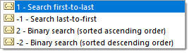
[search_mode]: Use 1 to search starting with the first item, and -1 to search starting from the last item. You can also use 2 to search a lookup_array sorted in acending order and -2 to sarch a lookup_array sorted in descending order (see about running binary searches in sorted arrays in our post about the DOUBLE VLOOKUP trick). The results returned will be invalid if the array is not sorted appropriately.
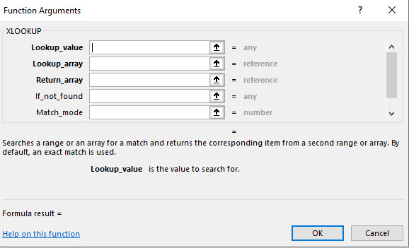
XLOOKUP function has 5 parameters, only the first 3 are required
Differences with examples
We are going to show some of differences between XLOOKUP and VLOOKUP functions [10].
XLOOKUP(lookup_value, lookup_array, return_array, [if_not_found], [match_mode], [search_mode])
1. Lookup to the left
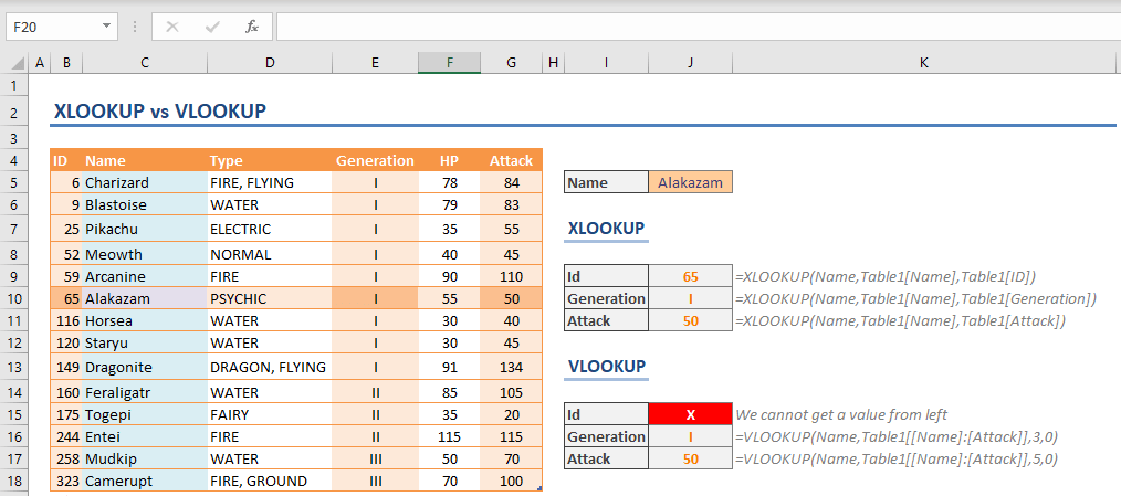
The first difference between XLOOKUP and VLOOKUP functions is the biggest limitation of the VLOOKUP: You can only search for a value in the left-most column of a table and retrieve a value from the columns to its right. A common workaround is using the INDEX-MATCH combination. With XLOOKUP you can get a value from any side of the search value.
Instead of selecting the entire range, the XLOOKUP requires 2 ranges:
- lookup_array: The array or range where you want to look up the value
- return_array: The array or range where you want to return a value from
As a result, you can select search and lookup ranges separately. In the following example, the formula searches for “Alakazam” in the Name column (Table13[Name]) and returns the ID value (Table13[ID]) matching the name.
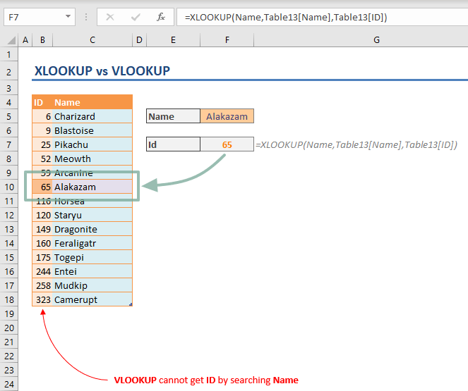
source: spreadsheetweb [10]
2. No column index
The col_index_num argument which determines the index of the return column for VLOOKUP. The XLOOKUP function, however, doesn’t need a parameter for counting columns.
Column index number can be tricky to determine for large tables. Furthermore, deleting a column can change indexes of each column after the deleted one. For example, if you delete the 3rd column from a 5-column table, the previous 4th and 5th columns will become 3rd and 4th.
You can see the argument differences between XLOOKUP and VLOOKUP below.
source: spreadsheetweb [10]
3. Match type
The default match type is “exact match” in XLOOKUP. VLOOKUP requires this to be defined with the range_lookup argument.
The XLOOKUP contains a similar argument named match_type as well. A 0 value here will make the function work like VLOOKUP.
Approximate match types
VLOOKUP’s range_lookup argument can have 2 values:
- 1: returns the value corresponding to the next smaller value if the search value does not exist
- 0: returns the corresponding value only if the search value exists
The XLOOKUP’s match_type has the additional options below:
- -1: returns the value corresponding to the next smaller if the search value does not exist
- 0: returns the corresponding value only if the search value exists
- 1: returns the value corresponding to the next greater if the search value does not exist
- 2: wildcard support
Thus, range_lookup = 1 works the same way as match_type = -1. VLOOKUP has wildcard support, and with the XLOOKUP, you can choose to include this as well.
Another improvement on approximate search is that you do not need to sort your data beforehand. Let’s take the example below. Both the XLOOKUP and the VLOOKUP are doing an approximate search. However, the VLOOKUP returns #N/A because the data is not sorted.
 source: spreadsheetweb [10]
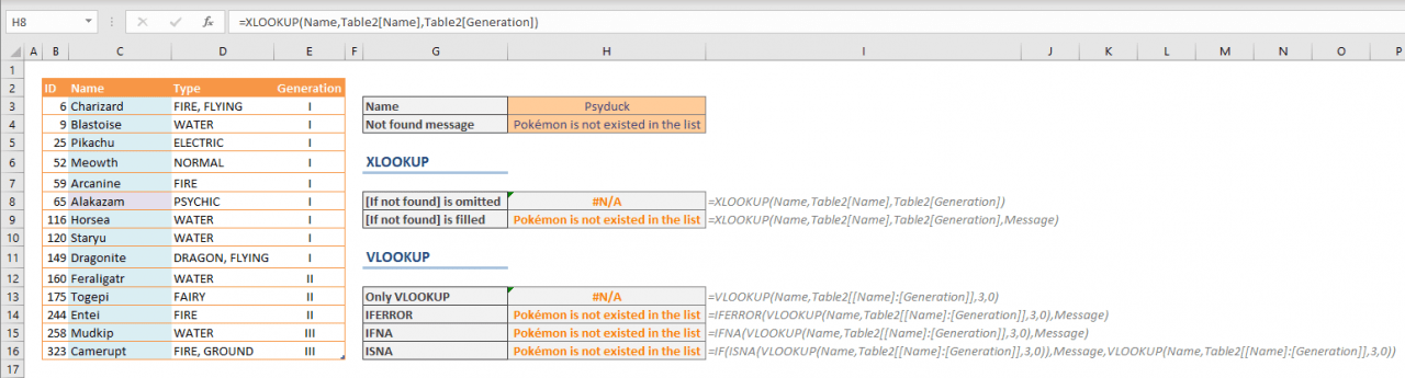
4. If not found
Thanks to the XLOOKUP’s if_not_found argument, you do not need to use other functions like IFERROR or IFNA to handle scenarios where no matches are found.
Please note that the XLOOKUP function is currently only accessible for Microsoft 365 subscribers.
 source: spreadsheetweb [10]
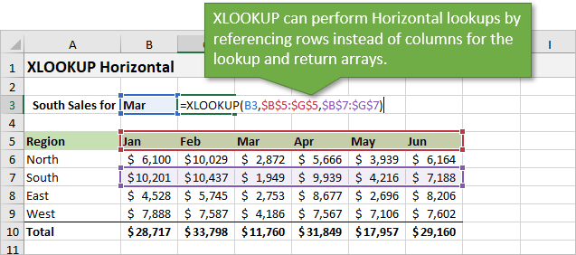
5. Horizontal Lookups
XLOOKUP can also do a horizontal lookup. We don’t need a separate function like HLOOKUP for this. You just specify single rows (instead of columns) for the lookup and return arrays.[12]
13 XLOOKUP Examples
We will use the [Sales] table data shown below [8]. Download Sample worksheet xlookup 13 examples
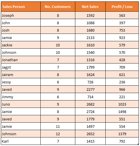
All the examples are listed in this table. Browse it and feel free to copy the formulas to test [8].
Note about references in the formula:
- Input or search values are in column H. The value used for searching is shown in first column. I used references rather than hardcoded values to make the formula relateable.
- Search is done against Sales Table as shown above.
| Criteria | Question | Answer | Formula | Notes |
|---|---|---|---|---|
| Jackie | What is the net sales? | 1610 | XLOOKUP(H5,sales[Sales Person],sales[Net Sales]) | Nice and simple. Finds H5 (Jackie) in the sales[Sales Person] list and returns macthing [Net Sales] if found. |
| 2133 | Whose sales are this? | Jamie | XLOOKUP(H6,sales[Net Sales],sales[Sales Person]) | This time, we lookup in the middle but return the name at front. Normally we would use INDEX+MATCH for something like this, but XLOOKUP just kills it. |
| Who has most sales? | Jamie | XLOOKUP(MAX(sales[Net Sales]),sales[Net Sales],sales[Sales Person]) | Of course, we can mix formulas too. MAX() finds the maximum sales and then XLOOKUP does the rest. Try other formulas like MIN(), SMALL(), LARGE() too. | |
| 8 | Who has this many customers? | Joseph | XLOOKUP(H8,sales[No. Customers],sales[Sales Person]) | Another example with find the middle, return from front. |
| 8 | Who is the last person to have this many customers? | Jamie | XLOOKUP(H9,sales[No. Customers],sales[Sales Person],,0,-1) | Now we are talking!!!, you can use the optional parameters for XLOOKUP to specify match type (0 is for exact match) and match direction (-1 is for bottom to top). |
| 1800 | Whose sales are closest to this number, but not more? | Jagjit | XLOOKUP(H10,sales[Net Sales],sales[Sales Person],”value not found”,-1) | We can search for a value that is closest but not more by using match type -1. |
| Ju | What is the profit of person whose name begins with this? | 1023 | XLOOKUP(H11&”*”,sales[Sales Person],sales[Profit / Loss],,2) | You can do wild card searches too. * for any number of letters and ? for single letter. |
| Who has least sales? | Jimmy | XLOOKUP(0,sales[Net Sales],sales[Sales Person],,1) | Time for a trick!!! When searching fields like [Net Sales] which will usually have just positive values, you can look for 0 with match type as 1 (next highest value). | |
| What is the sales for very last person? | 1415 | XLOOKUP(“*”,sales[Sales Person],sales[Net Sales],,2,-1) | Another trick! Search for “*” from end to get the last value’s matching sales. | |
| Who is the very last person? | Karl | XLOOKUP(“*”,sales[Sales Person], sales[Sales Person],,2,-1) | Of course, you can search and return from the same column to find out the last person’s name. | |
| Net Sales | What is H11 for Johnson? | 1540 | XLOOKUP(“Johnson”,sales[Sales Person],XLOOKUP(H15,sales[#Headers],sales)) | 2 way lookups by nesting XLOOKUP. Remember, inner XLOOKUP returns a list of [Net Sales] |
| Jamie | What is the Net Sales for second person with this name? | 2724 | XLOOKUP(H16&”2″,FILTER(sales[Sales Person],sales[Sales Person]=H16)&SEQUENCE(3),FILTER(sales[Net Sales],sales[Sales Person]=H16)) | You can combine XLOOKUP with other new formulas like FILTER() to create something crazy and fun too. Try it yourself. |
| Chandoo | What is the net sales? | Value not found | XLOOKUP(H17,sales[Sales Person],sales[Net Sales],”Value not found”) | And of course, when the data can’t be found XLOOKUP simly #N/As. To prevent this, you can use the 4th parameter to specify output value. |
Download another sheet for XLOOKUP training; wtf-xlookup
Please note that the XLOOKUP function is currently only accessible for Microsoft 365 subscribers.
More Emaples
Example 1
Here is how XLOOKUP looks in its simplest form: As you can see below, XLOOKUP is used in G2 to display a country telephone prefix based on the user input in F2.
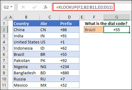
source: Microsoft Support [11]
With XLOOKUP we are getting the best of 2 worlds: like VLOOKUP it is very simple to type and remember, and like INDEX/MATCH the lookup_array is a reference that makes it more flexible. And icing on the cake, you don’t need to specify the match_mode to get an exact match.
XLOOKUP uses a lookup array and a return array, whereas VLOOKUP uses a single table array followed by a column index number. The equivalent VLOOKUP formula in this case would be: =VLOOKUP(F2,B2:D11,3,FALSE)
Now let’s see how you can use those scary optional arguments to make some awesome formulas.
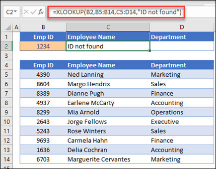
Example 2
This example adds an if_not_found argument to the preceding example. Below, the if_not_found argument is used to add a custom error message:
source: Microsoft Support [11]
That’s much clearer than getting #N/A results that people are not always sure how to interprete.
In this example, the if_not_found argument is text. But you can also return a value or a range. In many cases, it saves you the effort of combining VLOOKUP with IF, IFERROR or other formulas to handle the absence of match.
Example 3
Below, all 3 optional arguments are used:
-
The if_not_found argument is used, returning a value of 0 instead of #N/A if no match is found.
-
The match_mode argument is used, set to 1, so it’s looking for an exact match or the next larger item.
-
The search_mode argument is also used, set to 1, so searching starting from the first item down to the last.

source: Microsoft Support [11]
XARRAY’s lookup_array column is to the right of the return_array column, whereas VLOOKUP can only look from left-to-right.
Example 4
In the below example, XLOOKUP is being used to search for and display an employee’s information based on their ID.
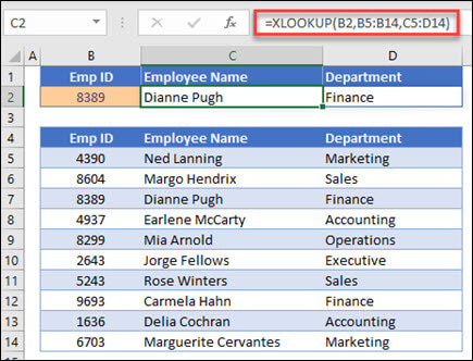
source: Microsoft Support [11]
XLOOKUP is displaying both the Employee Name in C2 and the Department in D2, with one single formula.
This is because XLOOKUP is able to return arrays with multiple items. This is very powerful, and a great time-saver if you need to get data from many columns.
Pay attention to the 3rd argument (the return_array argument). You would typically expect it to be C5:C14, but instead it’s C5:D14, meaning that the results will come from both the C and D columns!
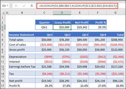
Example 5
This example uses a nested XLOOKUP function to perform both a vertical and horizontal match. It first looks for Gross Profit in column B, then looks for Qtr1 in the top row of the table (range C5:F5), and finally returns the value at the intersection of the two. This is similar to using the INDEX and MATCH functions together.[11]
source: Microsoft Support [11]
Note: The formula in cells D3:F3 is:
=XLOOKUP(D2,$B6:$B17,XLOOKUP($C3,$C5:$G5,$C6:$G17))
Example 6
This example uses the SUM function, and two nested XLOOKUP functions, to sum all the values between two ranges. In this case, we want to sum the values for grapes, bananas, and include pears, which are between the two.[11]
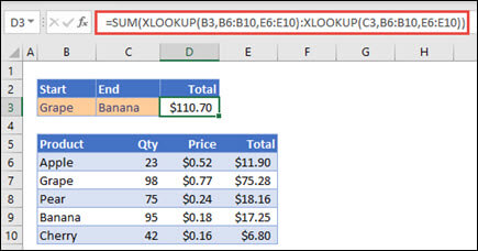
source: Microsoft Support [11]
The formula in cell E3 is:
=SUM(XLOOKUP(B3,B6:B10,E6:E10):XLOOKUP(C3,B6:B10,E6:E10))
How does it work? XLOOKUP returns a range, so when it calculates, the formula ends up looking like this: =SUM($E$7:$E$9). You can see how this works on your own by selecting a cell with an XLOOKUP formula similar to this one, then select Formulas > Formula Auditing > Evaluate Formula, and then select Evaluate to step through the calculation.[11]
xlookup vs vlookup vs index/match
Let’s recap how XLOOKUP outperforms VLOOKUP and INDEX/MATCH:[10]
- It is the simplest function, with only 3 arguments needed in most cases because the default match mode is 0 (exact match).
- It’s a single function, unlike INDEX/MATCH, so it’s faster to type.
- It works both vertically and horizontally (unlike VLOOKUP and its alter ego HLOOKUP).
- It doesn’t require the lookup values to be on the left (unlike VLOOKUP).
- It can return custom results instead of #N/A when no match is found, without needing to combine additional functions.
- It can return an array, and not just a single value.
- It can do binary searches to calculate faster on sorted data when [search mode] is -2 or 2.
- It can run partial searches, leveraging wildcard characters when [match mode] is 2.
- It can run reverse searches when [search mode] is -1.
Pros & Cons of XLOOKUP
XLOOKUP is an amazing new function and definitely has some major advantages over VLOOKUP and INDEX MATCH. It does have some drawbacks too.[12]
Pros or Advantages
Here is the list of advantages for XLOOKUP that I shared in the video above.
- Defaults to exact match.
- It only requires three arguments, instead of four for VLOOKUP or INDEX MATCH.
- Works both vertically and horizontally.
- One function instead of two, compared to INDEX MATCH.
- Can do partial match lookups with wildcard characters (4th argument = 2).
- Can do lookups in reverse order (5th argument = -1).
- Returns a range instead of a value (advanced nested formulas).
Cons or Drawbacks
There are also a few potential issues to be aware of.
- Additional [optional] arguments can make the function look overwhelming to new users.
- Returns a #VALUE! error if the lookup and return arrays are not the same length. I explain this in the video above.
- It can be time-consuming to select two ranges with the mouse, especially when you have thousands of cells in the arrays.
- You must remember to make both the lookup and return ranges absolute references (F4 on the keyboard) if copying the formula down/across.
- You must use nested functions to do a 2-dimensional lookup. Can use two XLOOKUPs or INDEX MATCH.
Summary and tips
- You can make right-to-left lookups with XLOOKUP.
- Adding or removing columns do not affect XLOOKUP.
- Approximate search can work both ways.
- No need to sort data for approximate search.
- You can determine search direction.
- The XLOOKUP doesn’t need entire table to be referenced – only search and return columns.
Excel supports VLOOKUP, HLOOKUP, and LOOKUP functions for backwards compatibility, but the new lookup formula can replace them all, and offers more functionality.
Conclusion
So there you have it, a breakdown of XLOOKUP vs VLOOKUP.
The XLOOKUP is a definite improvement to the VLOOKUP and replaces a lot of the bypasses that you had to rely on to get a VLOOKUP to work in certain instances (INDEX, MATCH, IFERROR, and other maneuverings).
The XLOOKUP is unfortunately not available for older versions of Excel, and you will have to keep this in mind when sharing worksheets.
VLOOKUP was a trusted old companion and it may still have a place in certain instances – so don’t write it off yet. But the XLOOKUP is without a doubt a great and much-needed improvement.